Applying the gradient descent algorithm to find the minimum of the following function of four variables

Introduction
Gradient is an algorithm used to find the parameters that minimizes a function. We will be using the function above to implement gradient descent. To implement a gradient descent algorithm there are some important ingredients to be used which includes;
- The function
- The partial derivative of all the function
The gradient descent algorithm finds the best path to descend to the minimum points in a function by finding the slope of the tangent of the function. We will be implementing the batch gradient descent algorithm in this task. The slope of the tangent tells us the direction of our descent.
Gradient descent procedure
The algorithm starts off with initial values for the parameters of the function. These could be 0.0 or a small random value. We observed that using zero initialization for this algorithm makes it impossible for us to update some of the parameters such as (w and z) due to the exponentials. We initiated the algorithm using random initialization to solve this problem.
The cost of the parameters is evaluated by inserting them into the function and calculating the cost of using this parameters.
The derivative of the function is calculated. The derivative of the function as stated above is the slope of the function. We need to know the slope so that we know the direction (sign) to move the parameter values in order to get a lower cost on the next iteration.
Now that we know direction or slope of the function, we can now update the parameter values. We used the learning rate to state the size of the step to take during each iteration.
This process is repeated until the cost of the parameters close to zero or minimum enough.
Finding the partial derivative of independent variables in equation above
we will be applying the partial derivative, power rule and chain rule to the function above.


After finding the derivative of the function with respect to each element in the equation, we created a function “fun” which returns the result of the original equation whenever we give it inputs as argument. We then proceeded to create a function for each of the partial derivatives as this would be used when implementing the gradient descent algorithm. We added a tolerance of 0.01 and step seize of 0.03.
import numpy as np
import math
import matplotlib.pyplot as plt
import seaborn as sns
import random
import pandas as pd

%matplotlib inline
random.seed(20210402)
x=random.random()
y=random.random()
z=random.random()
w=random.random()
#partial derivative (1/4(2-x)^2) + (3y-5)^4 + e^(2z^4 + w^2)

#define the function
def fun(x,y,z,w):
    return  ((1/4)*(2-x)**2) + ((3*y)-5)**4 + math.exp((2*(z**4))+(w**2))

#define the derivative w.r.t x
def der_x(x):
    return (x-2)/2

#define the derivative w.r.t y
def der_y(y):
    return 12*((3*y)-5)**3

#define the derivative w.r.t z
def der_z(z,w):
    return ((8)*(z**3))*math.exp((2*(z**4))+(w**2))

#define the derivative w.r.t w
def der_w(w,z):
    return (2*w)*math.exp((2*(z**4))+(w**2))

#define the grad descent
def step(init_param,grad,step_size):
    return (init_param - (step_size * grad))

#define the counter
i = 0

#define the tolerance
tolerance = 0.01
step_size = 0.03

#create an empty list
my_list =[]

#loop till we find the minimum point
while True:
    i +=1
    #print(x,y,z,w,fun(x,y,z,w))
    my_list.append([x,y,z,w,fun(x,y,z,w)])

    #assign derivative of each parameter
    grad_x = der_x(x)
    grad_y = der_x(y)
    grad_z = der_z(z,w)
    grad_w = der_w(w,z)

    #apply the step function
    next_x = step(x, grad_x, step_size)
    next_y = step(y, grad_y, step_size)
    next_z = step(z, grad_z, step_size)
    next_w = step(w, grad_w, step_size)

    #apply tolerance to break out of the loop
    if (np.sqrt(((x-next_x)**2 + (y-next_y)**2 +  (z-next_z)**2 + (w-next_w)**2)) < tolerance):
        break

    #assign output to variables x,y,z,w
    x,y,z,w= next_x,next_y,next_z,next_w

print("It took {} epochs, for the algorithm to find the minimum point".format(i))

#load the independent variables into a dataaframe
parameters = pd.DataFrame(np.array(my_list), columns = ['x','y','z','w','cost_fun'])
parameters['zero'] = pd.Series([0 for x in range(len(parameters.index))], index=parameters.index)
It took 67 epochs, for the algorithm to find the minimum point
It was observed that the alorithm took 67 iterations to find the parameters that minimizes our function, the initial values of the parameter influences gradient descent and how long it takes to descend, if we change the step size and parameter initiation we would observe the number of iteration required to converge at the local optima would be different from what we currently have.
parameters.head()
.dataframe tbody tr th {
    vertical-align: top;
}

.dataframe thead th {
    text-align: right;
}
parameters.tail()
.dataframe tbody tr th {
    vertical-align: top;
}

.dataframe thead th {
    text-align: right;
}
import plotly.graph_objects as go

fig = go.Figure(data =
    go.Contour(
        x=parameters.x, # horizontal axis
        y=parameters.y, # vertical axis
        z=parameters.cost_fun,
        colorscale='Electric',

    ))
fig.show()

import plotly.graph_objects as go

fig = go.Figure(data =
    go.Contour(
        x=parameters.z, # horizontal axis
        y=parameters.w, # vertical axis
        z=parameters.cost_fun,
        colorscale='Electric',

    ))
fig.show()

from plotly.subplots import make_subplots
import plotly.graph_objects as go

fig = go.Figure()

fig.add_trace(go.Scatter3d(x=parameters.x, y=parameters.zero, z=parameters.cost_fun,    mode="markers+text",
    name="Markers and Text",
    text=["X"],
    textposition="bottom center"))
fig.add_trace(go.Scatter3d(x=parameters.y, y=parameters.zero, z=parameters.cost_fun,    mode="markers+text",
    name="Markers and Text",
    text=["Y"],
    textposition="bottom center"))
fig.add_trace(go.Scatter3d(x=parameters.z, y=parameters.zero, z=parameters.cost_fun,    mode="markers+text",
    name="Markers and Text",
    text=["Z"],
    textposition="top center"))
fig.add_trace(go.Scatter3d(x=parameters.w, y=parameters.zero, z=parameters.cost_fun,    mode="markers+text",
    name="Markers and Text",
    text=["W"],
    textposition="top center"))


fig.update_layout(showlegend=False,
    title="3D Plot gradient descent",
    font=dict(
        family="Courier New, monospace",
        color="RebeccaPurple"
    )
)


fig.show()
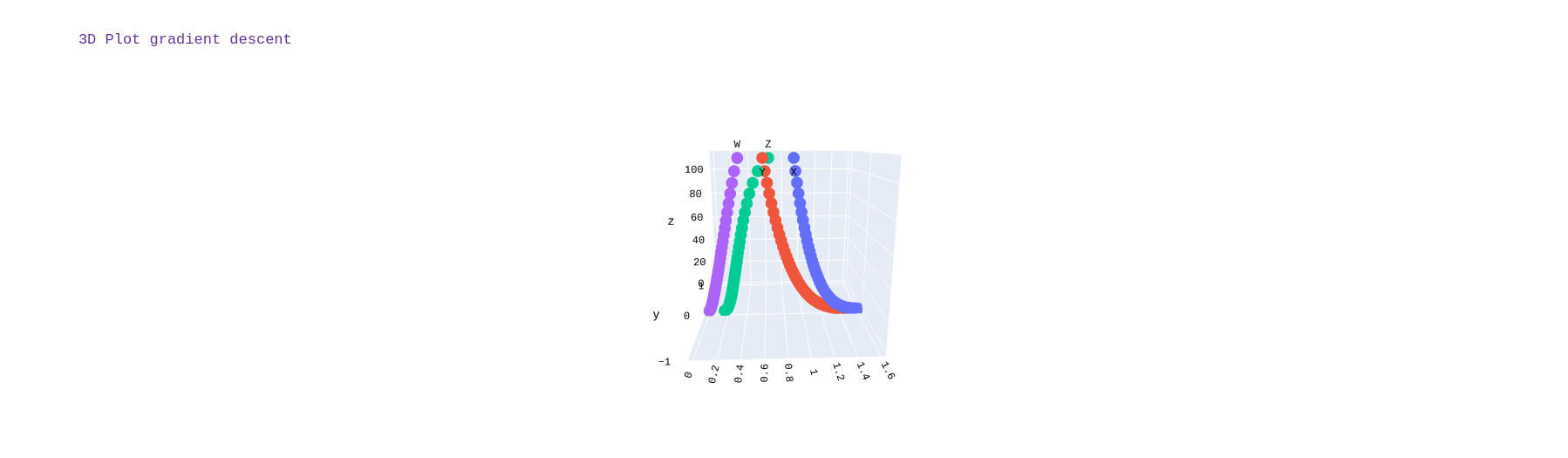
Results
Visualizing the outcome of the implementation of the gradient descent algorithm we can observe that gradient descent was able to find the parameters that minimizes the cost function, we used random initialization for selecting the initial starting points to avoid the saturation of our cost function as we observed that using zero initialization makes it impossible for the gradient descent algorithm to update the parameters z and w. The plot for the path taken by the algorithm for the simulataneus update for all the parameters is different but we can observe they all converge at the same value of the cost function regardless of the path taken.The visualization showed that the path taken by variables x and y is different to that which z and w took, but we observe that they all eventually converge at the local optima.